[R]Hydromad on Cikapundung-update on monthly analysis

After discussing my codes on the previous post about using Hydromad to Cikapundung dataset, It turned out that the codes were for daily analysis. Where as to convert it to monthly analysis, we should set the warm up and objective function.

We add:

• hydromad.options(warmup=12) to set montly analysis
• objective=~hmadstat("r.squared") to use Nash-Sutcliffe Efficiency/NSE as the objective function for our calibration.

Then the whole code will look like this,

# open hydromad
library(hydromad)
setwd("~/R practice-cikapundung")

# load data (flow, rain, temp)
Flow <- read.csv("flowlembang2.csv")
head(Flow)

##       Date Flow
## 1 1/1/2007 2.57
## 2 1/2/2007 2.57
## 3 1/3/2007 2.50
## 4 1/4/2007 2.44
## 5 1/5/2007 2.41
## 6 1/6/2007 2.39

Rain <- read.csv("rainlembang.csv")
head(Rain)

##       Date  Rain
## 1 1/1/2007 2.000
## 2 1/2/2007 2.000
## 3 1/3/2007 2.125
## 4 1/4/2007 2.250
## 5 1/5/2007 2.375
## 6 1/6/2007 2.500

Temp <- read.csv("templembang.csv")
head(Temp)

##       Date MaxT
## 1 1/1/2007 18.9
## 2 1/2/2007 18.4
## 3 1/3/2007 18.3
## 4 1/4/2007 17.9
## 5 1/5/2007 19.6
## 6 1/6/2007 20.2

# Convert the date column
Flow$Date <- as.Date(Flow[, 1], "%m/%d/%Y")
Rain$Date <- as.Date(Rain[, 1], "%m/%d/%Y")
Temp$Date <- as.Date(Temp[, 1], "%m/%d/%Y")

# use package zoo
library(zoo)
tsQ <- zoo(Flow$Flow, order.by = Flow$Date, frequency = 1)
tsP <- zoo(Rain$Rain, order.by = Rain$Date, frequency = 1)
tsT <- zoo(Temp$MaxT, order.by = Temp$Date, frequency = 1)

# merge data
Cikapundung <- merge(P = tsP, Q = tsQ, E = tsT, all = F)
head(Cikapundung)

##                P    Q    E
## 2007-01-01 2.000 2.57 18.9
## 2007-01-02 2.000 2.57 18.4
## 2007-01-03 2.125 2.50 18.3
## 2007-01-04 2.250 2.44 17.9
## 2007-01-05 2.375 2.41 19.6
## 2007-01-06 2.500 2.39 20.2

monthlyPQE <- aggregate(Cikapundung, as.yearmon, mean)

# model spec define data period name 'ts.cal', 'ts.val', 'ts.later' split
# the data into different sections
ts.cal <- window(Cikapundung, start = "2007-01-01", end = "2008-12-31")
ts.val <- window(Cikapundung, start = "2008-01-01", end = "2009-12-31")
ts.later <- window(Cikapundung, start = "2009-01-01", end = "2010-12-31")

# using monthly data with Armax and Expuh routing armax
hydromad.options(warmup = 12)
ckpModel.armax <- hydromad(ts.cal, sma = "cmd", routing = "armax", rfit = list("sriv", 
    order = c(n = 2, m = 1)))
ckpFit.armax.NSE <- fitByOptim(ckpModel.armax, objective = ~hmadstat("r.squared")(Q, 
    X), samples = 100, method = "PORT")

## Warning: did not converge after 12 iterations
## Warning: did not converge after 12 iterations
## Warning: did not converge after 12 iterations
## Warning: did not converge after 12 iterations
## Warning: did not converge after 12 iterations
## Warning: did not converge after 12 iterations
## Warning: did not converge after 12 iterations
## Warning: did not converge after 12 iterations
## Warning: did not converge after 12 iterations
## Warning: did not converge after 12 iterations
## Warning: did not converge after 12 iterations
## Warning: did not converge after 12 iterations
## Warning: did not converge after 12 iterations
## Warning: did not converge after 12 iterations
## Warning: did not converge after 12 iterations
## Warning: did not converge after 12 iterations
## Warning: did not converge after 12 iterations
## Warning: did not converge after 12 iterations
## Warning: did not converge after 12 iterations
## Warning: did not converge after 12 iterations
## Warning: did not converge after 12 iterations
## Warning: did not converge after 12 iterations
## Warning: did not converge after 12 iterations
## Warning: did not converge after 12 iterations
## Warning: did not converge after 12 iterations
## Warning: did not converge after 12 iterations
## Warning: did not converge after 12 iterations
## Warning: did not converge after 12 iterations
## Warning: did not converge after 12 iterations
## Warning: did not converge after 12 iterations
## Warning: did not converge after 12 iterations
## Warning: did not converge after 12 iterations
## Warning: did not converge after 12 iterations
## Warning: did not converge after 12 iterations
## Warning: did not converge after 12 iterations
## Warning: did not converge after 12 iterations
## Warning: did not converge after 12 iterations
## Warning: did not converge after 12 iterations
## Warning: did not converge after 12 iterations
## Warning: did not converge after 12 iterations
## Warning: did not converge after 12 iterations
## Warning: did not converge after 12 iterations
## Warning: did not converge after 12 iterations
## Warning: did not converge after 12 iterations
## Warning: did not converge after 12 iterations
## Warning: did not converge after 12 iterations
## Warning: did not converge after 12 iterations
## Warning: did not converge after 12 iterations
## Warning: did not converge after 12 iterations
## Warning: did not converge after 12 iterations
## Warning: did not converge after 12 iterations
## Warning: did not converge after 12 iterations
## Warning: did not converge after 12 iterations
## Warning: did not converge after 12 iterations
## Warning: did not converge after 12 iterations
## Warning: did not converge after 12 iterations
## Warning: did not converge after 12 iterations
## Warning: did not converge after 12 iterations
## Warning: did not converge after 12 iterations
## Warning: did not converge after 12 iterations
## Warning: did not converge after 12 iterations
## Warning: did not converge after 12 iterations
## Warning: did not converge after 12 iterations
## Warning: did not converge after 12 iterations
## Warning: did not converge after 12 iterations
## Warning: did not converge after 12 iterations
## Warning: did not converge after 12 iterations
## Warning: did not converge after 12 iterations
## Warning: did not converge after 12 iterations
## Warning: did not converge after 12 iterations
## Warning: did not converge after 12 iterations
## Warning: did not converge after 12 iterations
## Warning: did not converge after 12 iterations
## Warning: did not converge after 12 iterations
## Warning: did not converge after 12 iterations
## Warning: did not converge after 12 iterations
## Warning: did not converge after 12 iterations
## Warning: did not converge after 12 iterations
## Warning: did not converge after 12 iterations
## Warning: did not converge after 12 iterations
## Warning: did not converge after 12 iterations
## Warning: did not converge after 12 iterations
## Warning: did not converge after 12 iterations
## Warning: did not converge after 12 iterations
## Warning: did not converge after 12 iterations
## Warning: did not converge after 12 iterations
## Warning: did not converge after 12 iterations
## Warning: did not converge after 12 iterations
## Warning: did not converge after 12 iterations
## Warning: did not converge after 12 iterations
## Warning: did not converge after 12 iterations
## Warning: did not converge after 12 iterations
## Warning: did not converge after 12 iterations
## Warning: did not converge after 12 iterations
## Warning: did not converge after 12 iterations
## Warning: did not converge after 12 iterations
## Warning: did not converge after 12 iterations
## Warning: did not converge after 12 iterations
## Warning: did not converge after 12 iterations
## Warning: did not converge after 12 iterations
## Warning: did not converge after 12 iterations
## Warning: did not converge after 12 iterations
## Warning: did not converge after 12 iterations
## Warning: did not converge after 12 iterations
## Warning: did not converge after 12 iterations
## Warning: did not converge after 12 iterations
## Warning: did not converge after 12 iterations
## Warning: did not converge after 12 iterations
## Warning: did not converge after 12 iterations
## Warning: did not converge after 12 iterations
## Warning: false convergence (8)

summary(ckpFit.armax.NSE)

## 
## Call:
## hydromad(DATA = ts.cal, sma = "cmd", routing = "armax", rfit = list("sriv", 
##     order = c(n = 2, m = 1)), f = 0.4026, e = 0.8829, d = 146)
## 
## Time steps: 719 (3 missing).
## Runoff ratio (Q/P): (3.92 / 9.34) = 0.419
## rel bias: -0.136
## r squared: -0.35
## r sq sqrt: -0.878
## r sq log: -0.878
## 
## For definitions see ?hydromad.stats

coef(ckpFit.armax.NSE)

##         f         e         d     shape       a_1       a_2       b_0 
##   0.40260   0.88290 146.00000   0.00000   1.98295  -0.98306   0.01065 
##       b_1     delay 
##  -0.01054   2.00000

print(ckpFit.armax.NSE)

## 
## Hydromad model with "cmd" SMA and "armax" routing:
## Start = 2007-01-01, End = 2008-12-31
## 
## SMA Parameters:
##       f        e        d    shape  
##   0.403    0.883  146.000    0.000  
## Routing Parameters:
##     a_1      a_2      b_0      b_1    delay  
##  1.9829  -0.9831   0.0107  -0.0105   2.0000  
## TF Structure: S + Q (two stores in parallel)
##     Poles:0.9915+0.0063i, 0.9915-0.0063i 
## 
## Fit: ($fit.result)
## fitByOptim(MODEL = ckpModel.armax, objective = ~hmadstat("r.squared")(Q, 
##     X), method = "PORT", samples = 100)
##      135 function evaluations in 11.37 seconds 
## 
## Routing fit info:  list(converged = FALSE, iteration = 12) 
## 
## Message: false convergence (8)

xyplot(ckpFit.armax.NSE, with.P = TRUE, type = c("l", "g"))

## expuh
hydromad.options(warmup = 12)
ckpModel.expuh <- hydromad(ts.cal, sma = "cwi", routing = "expuh", tau_s = c(5, 
    100), tau_q = c(0, 5), v_s = c(0, 1))
ckpFit.expuh.NSE <- fitByOptim(ckpModel.expuh, objective = ~hmadstat("r.squared")(Q, 
    X), samples = 100, method = "PORT")
summary(ckpFit.expuh.NSE)

## 
## Call:
## hydromad(DATA = ts.cal, tau_s = 100, tau_q = 2.9763, v_s = 0.892532, 
##     sma = "cwi", routing = "expuh", tw = 6.96977, f = 8, scale = 0.00547393)
## 
## Time steps: 719 (1 missing).
## Runoff ratio (Q/P): (3.92 / 9.32) = 0.421
## rel bias: 1.98e-17
## r squared: -0.303
## r sq sqrt: -0.534
## r sq log: -0.545
## 
## For definitions see ?hydromad.stats

coef(ckpFit.expuh.NSE)

##        tw         f     scale         l         p     t_ref     tau_s 
## 6.970e+00 8.000e+00 5.474e-03 0.000e+00 1.000e+00 2.000e+01 1.000e+02 
##     tau_q       v_s 
## 2.976e+00 8.925e-01

print(ckpFit.expuh.NSE)

## 
## Hydromad model with "cwi" SMA and "expuh" routing:
## Start = 2007-01-01, End = 2008-12-31
## 
## SMA Parameters:
##       tw         f     scale         l         p     t_ref  
##  6.96977   8.00000   0.00547   0.00000   1.00000  20.00000  
## Routing Parameters:
##   tau_s    tau_q      v_s  
## 100.000    2.976    0.893  
## TF Structure: S + Q (two stores in parallel)
##     Poles:0.7146, 0.99 
## 
## Fit: ($fit.result)
## fitByOptim(MODEL = ckpModel.expuh, objective = ~hmadstat("r.squared")(Q, 
##     X), method = "PORT", samples = 100)
##      221 function evaluations in 11.87 seconds

xyplot(ckpFit.expuh.NSE, with.P = TRUE, type = c("l", "g"))

You might also get the ## Warning: did not converge after 12 iterations. Please refer to the following discussion on hydromad user group. The fitByOptim command is the one that iterate the model equation with the best fit parameters. It saves us time for not have to re-input all the parameters from the print(xxxx), coef(xxx), or summary(xxx).

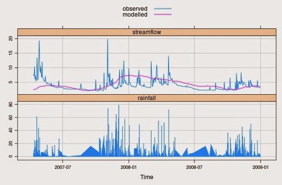
If we look at the plot, we would agree that both of the fitting (pink line) don't capture many parts of the observed data (blue line). However it is normal because we only had 4 years of data in total and only use one year (2007-2008) period as calibration data.

Additional reference:

• Jain, S. and Sudheer, K. (2008). “Fitting of Hydrologic Models: A Close Look at the Nash-Sutcliffe Index.” J. Hydrol. Eng., 13(10), 981-986.TECHNICAL NOTES, http://dx.doi.org/10.1061/(ASCE)1084-0699(2008)13:10(981)
• McCuen, R., Knight, Z., and Cutter, A. (2006). “Evaluation of the Nash-Sutcliffe Efficiency Index.” J. Hydrol. Eng., 11(6), 597-602. TECHNICAL PAPERS, http://dx.doi.org/10.1061/(ASCE)1084-0699(2006)11:6(597)

Good luck {@dasaptaerwin}

[R] Try out Armax and Expuh Routing

Try out Armax and Expuh Routing

This code is based on:

• Hydromad Tutorial by Felix Andrews
• Willem Vervoort class (LWSC3007)
• Discussion in Hydromad User Groups

Using armax

Code

ckpModel.armax <- hydromad(ts.cal,sma="cmd",routing="armax", 
                           rfit=list("sriv", order=c(n=2,m=1)))
ckpFit.armax <- fitByOptim(ckpModel.armax, samples=100, method="PORT")
summary(ckpFit.armax)
print(ckpFit.armax)
xyplot(ckpFit.armax, with.P=TRUE, type=c("l","g")) 

Results Summary

Call:
hydromad(DATA = ts.cal, tau_s = c(5, 100), tau_q = c(0, 5), v_s = c(0, 
    1), sma = "cmd", routing = "armax", rfit = list("sriv", order = c(n = 2, 
    m = 1)), f = 0.342265, e = 1.24435, d = 539.901)

Time steps: 631 (3 missing).
Runoff ratio (Q/P): (3.941 / 9.398) = 0.4194
rel bias: -0.07458
r squared: -0.3214
r sq sqrt: -0.3921
r sq log: -0.4041

print

Hydromad model with "cmd" SMA and "armax" routing:
Start = 2007-01-01, End = 2008-12-31

SMA Parameters:
       f         e         d     shape  
  0.3423    1.2444  539.9013    0.0000  
Routing Parameters:
     a_1       a_2       b_0       b_1     delay  
 1.92278  -0.92388  -0.01885   0.01995   2.00000  
TF Structure: S + Q (two stores in parallel)
    Poles:0.9415, 0.9813 

Fit: ($fit.result)
fitByOptim(MODEL = ckpModel, method = "PORT", samples = 100)
     173 function evaluations in 22.49 seconds 

Routing fit info:  list(converged = FALSE, iteration = 12) 

Message: false convergence (8) 

plot armax

Using expuh

Code

ckpModel.expuh <- hydromad(ts.cal,sma="cwi",routing="expuh",
                           tau_s=c(5,100),tau_q=c(0,5),v_s=c(0,1))
ckpFit.expuh <- fitByOptim(ckpModel.expuh, samples=100, method="PORT")
summary(ckpFit.expuh)
print(ckpFit.expuh)
xyplot(ckpFit.expuh, with.P=TRUE, type=c("l","g")) 

Results summary

all:
hydromad(DATA = ts.cal, tau_s = 100, tau_q = 1.60298, v_s = 0.921673, 
    sma = "cwi", routing = "expuh", tw = 6.42525, f = 8, scale = 0.00548436)

Time steps: 631 (1 missing).
Runoff ratio (Q/P): (3.947 / 9.38) = 0.4208
rel bias: 1.058e-16
r squared: -0.1464
r sq sqrt: -0.1787
r sq log: -0.1894

For definitions see ?hydromad.stats

print

Hydromad model with "cwi" SMA and "expuh" routing:
Start = 2007-01-01, End = 2008-12-31

SMA Parameters:
       tw          f      scale          l          p      t_ref  
 6.425251   8.000000   0.005484   0.000000   1.000000  20.000000  
Routing Parameters:
   tau_s     tau_q       v_s  
100.0000    1.6030    0.9217  
TF Structure: S + Q (two stores in parallel)
    Poles:0.5359, 0.99 

Fit: ($fit.result)
fitByOptim(MODEL = ckpModel.expuh, method = "PORT", samples = 100)
     204 function evaluations in 18.28 seconds 

plot expuh:


which one is the best fit?

[R] Hydromad for Cikapundung catchment analysis: An Exercise

Hydromad application to Cikapundung Catchment, West Java, Indonesia: An Exercise

An R Markdown document Author: Dasapta Erwin References: Hydromad Tutorial (by Feliz Andrews) and Hydrological Modeling Lecture Notes (by Willem Vervoort) Data prepared by: Ahmad Darul and Tata Setiawan

This file is an preliminary analysis on Cikapundung river dataset, a catchment in Bandung, West Java Province, Indonesia. The dataset is a four year data (2007, 2008, 2009, 2010) of daily river discharge, rainfall, and max temp.

Script header

# R script following Hydromad Tutorial by Felix Andrews
# link: http://hydromad.catchment.org/downloads/tutorial.pdf
# and Willem Vervoort's Class (lwsc3007)
# ------------------------------

Opening library and loading data

# open hydromad and set working dir
library(hydromad)
library(zoo)
setwd("/media/dasaptaerwin/DATA/BAPAK-2014/SYDNEY/Exercise/R practice-cikapundung")

# load data (flow, rain, temp)
Flow <- read.csv("flowlembang2.csv") 
head(Flow)
Rain <- read.csv("rainlembang.csv")
head(Rain)
Temp <- read.csv("templembang.csv")
head(Temp)

Converting date format in date column in each csv file. This important since it can be the source of many error messages, especially in plot and zoo commands.

# Convert the date column
Flow$Date <- as.Date(Flow[,1], "%m/%d/%Y")
Rain$Date <- as.Date(Rain[,1],"%m/%d/%Y")
Temp$Date <- as.Date(Temp[,1],"%m/%d/%Y")

Ordering data based on date with zoo package, and then merge it in to Cikapundung data frame.

# use package zoo
tsQ <- zoo(Flow$Flow,order.by=Flow$Date,frequency=1)
tsP <- zoo(Rain$Rain,order.by=Rain$Date,frequency=1)
tsT <- zoo(Temp$MaxT,order.by=Temp$Date,frequency=1)

# merge data
Cikapundung <- merge(P=tsP, Q=tsQ, E=tsT, all=F)

Be sure to check your data frame with head(data.frame) command to see if your date is in order, with P, Q, E column in it. My previous failure starts with ignoring this check. If it's not in order, for instance: there are only two columns instead of three, then you should check your csv file. Then re-run every lines.

> head(Cikapundung)
               P    Q    E
2007-01-01 2.000 2.57 18.9
2007-01-02 2.000 2.57 18.4
2007-01-03 2.125 2.50 18.3
2007-01-04 2.250 2.44 17.9
2007-01-05 2.375 2.41 19.6
2007-01-06 2.500 2.39 20.2

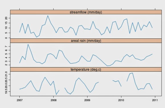
Then ordering your data in monthly basis and plot it.

monthlyPQE <- aggregate(Cikapundung, as.yearmon, mean)
xyplot(monthlyPQE, screens=c("streamflow (mm/day)", 
                          "areal rain (mm/day)", "temperature (deg.c)"), xlab=NULL)

Your output should look like this.

You can also check your complete cases and Runoff Ratio (RR)

ok <- complete.cases(Cikapundung[,1:2])
count(ok==T)
sum(Cikapundung$Q[ok])/sum(Cikapundung$P[ok])

The result should be.

     x freq
1 TRUE 1461

and

[1] 0.3672767

Next is calculating the correlation between river discharge (flow) and rainfall with rollccf function and estimating the delay.

r_ccf <- rollccf(Cikapundung)
plot(r_ccf$rolls$"width 365")

# Estimate delay time from rainfall to river
delay <- estimateDelay(Cikapundung)
delay

It should look like this,

and

> delay <- estimateDelay(Cikapundung)
> delay
[1] 2

Now we put in the model spec by defining define data period name ts.cal(calibration period), ts.val, and ts.later as testing period.

ts.cal <- window(Cikapundung,start="2007-01-01",end="2008-12-31")
ts.val <- window(Cikapundung,start="2008-01-01",end="2009-12-31")
ts.later <- window(Cikapundung,start="2009-01-01",end="2010-12-31")

Then defining routing and parameters using:

• ts.cal period
• expuh routing
• cwi (catchment wetness index) as sma (soil moisture accounting)
• tau_s=5-100 (slow flow component),
• tau_q=0-5 (fast flow component),
• v_s=0-1 (fraction volume in slow component)

ckpModel <- hydromad(ts.cal,sma="cwi",routing="expuh",tau_s=c(5,100),tau_q=c(0,5),v_s=c(0,1))
print(ckpModel)
out<-capture.output(print(ckpModel)) # saving result to txt file
cat(out,file="ckpModel1.txt",sep="\n",append=TRUE)

The output should look like this.

Hydromad model with "cwi" SMA and "expuh" routing:
Start = 2007-01-01, End = 2008-12-31

SMA Parameters:
      lower upper     
tw        0   100     
f         0     8     
scale    NA    NA     
l         0     0 (==)
p         1     1 (==)
t_ref    20    20 (==)
Routing Parameters:
      lower upper  
tau_s     5   100  
tau_q     0     5  
v_s       0     1  

Model calibration using fitByOptim function.

ckpModel <- update(ckpModel, sma="cmd", routing="armax", rfit=list("sriv", order=c(n=2,m=1)))
ckpFit <- fitByOptim(ckpModel, samples=100, method="PORT")

If you get error messages like subset out of bound etc, most likely you have problem with you data (eg: date format etc).

Then we try to simulate other period ts.val and ts.later,

simval <- update(ckpFit, newdata=ts.val)
simlater <- update(ckpFit, newdata=ts.later)

then running verification towhole dataset, excluding calib data.

dataVerif <- Cikapundung # make dataVerif frame from Cotter
dataVerif$Q[time(ts.cal)] <- NA # we verify Q and excluding data90ss 
simVerif <- update(ckpFit, newdata=dataVerif) # run dataVerif, save in simVerif

Next we can group all models using runlist function and save it in txt file,

allModels <- runlist(calibration=ckpFit, simval, simlater, simVerif)
summary(allModels) # summary of model performance
print(allModels)
out<-capture.output(print(allModels))
cat(out,file="allModels.txt",sep="\n",append=TRUE)

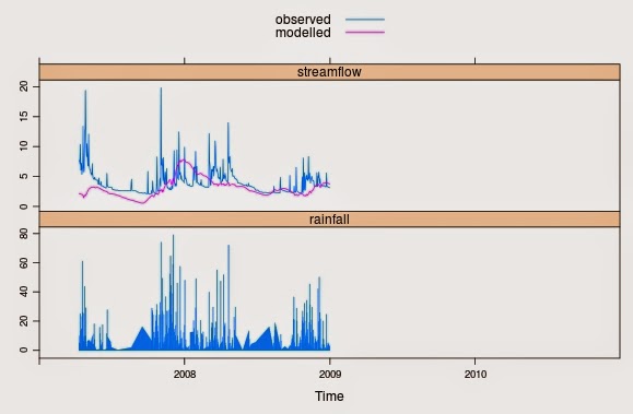
plotting ckpFit with defined period,

xyplot(ckpFit, with.P=TRUE, xlim=as.Date(c("2007-01-01", "2010-12-31")))

It should look like this.

and plotting allModels

xyplot(allModels[2:3], scales = list(y = list(log = TRUE)))

It should look like this.

The allModels summary should look like this.

         rel.bias    r.squared   r.sq.sqrt    r.sq.log
calibration -0.2168151 -0.380018043 -0.60152528 -0.64466581
simval       0.1793397 -0.524916565 -0.68196244 -0.73832646
simlater     0.5275161 -2.195907097 -1.63192686 -1.45632787
simVerif     0.1042556 -0.003519501  0.06358249  0.08402725

[R] How to compile R package (Hydromad) on Mavericks

[R] Hey R, may I introduce you to Mavericks :-)

I was noticing that R and Mavericks doesn't work-well together. It's because Mavericks keeps using its own new compiler from Xcode 5xx, that different from the standard R package compiler (pls CMIIW). Then install.package command won't work in this situation, including for Hydromad.

So for those of you that mistakenly have upgraded the OS to Mavericks, you have to introduce the right compiler for R package to Mavericks. So it will use it whenever you run install.package command. Thanks to StackOverflow Q&A.

First: You have to download the Xcode 5 from Appstore. It should be properly installed in you Mac. So you don't have to run it.

Second: Run the "terminal' window. The icon should be in your "Utility" program group. The one in the middle.

If your run it the a window like this will open

Third: Then on the terminal prompt type the following code (press "return" after each line):

cd /usr/bin
sudo ln -fs clang llvm-gcc-4.2
sudo ln -fs clang++ llvm-g++-4.2

After that, you should close everything then restart your MBA.

Then you can try again the process to install.package in R from tar.gz file.

Hope it helps. It works on my friend's MBA running Mavericks.

[R] Following Hydromad Tutorial

(Cotter Catchmen map)

The following is the code, following Hydromad Tutorial by Felix Andrews.

---
# R script following Hydromad Tutorial by Felix Andrews
# link: http://hydromad.catchment.org/downloads/tutorial.pdf
# ------------------------------

# open hydromad
library(hydromad)

# open data
data(Cotter)

# checking data
xyplot(Cotter, screens=c("streamflow (mm/day)", 
                         "areal rain (mm/day)", 
                         "temperature (deg.c)"), xlab=NULL)
xyplot(window(Cotter, start="1974-01-01", 
              end="1975-01-01"))
monthlyPQE <- aggregate="" as.yearmon="" font="" mean="" otter="">
xyplot(monthlyPQE, screens=c("streamflow (mm/day)", 
                             "areal rain (mm/day)", "temperature (deg.c)"), xlab=NULL)
ok <- 1:2="" complete.cases="" font="" otter="">
with(Cotter, sum(Q[ok])/sum(P[ok]))
head(Cotter)
tail(Cotter)


# calculate rolling cross-correlation
# between rainfall and streamflow rises
# from 1980 to 1990 data period
x <- font="" otter="" rollccf="">
xyplot(x, xlim=extendrange(as.Date(c("1980-01-01", 
                                     "1990-01-01"))))

# estimateDelay(x)
delay <- estimatedelay="" font="" otter="">
delay

# model spec
# define data period name "data70s", "data80s", "data90s"
data70s <- font="" nbsp="" otter="" start="1970-01-01" window="">
                  end="1979-12-31")
data80s <- font="" nbsp="" otter="" start="1980-01-01" window="">
                  end="1989-12-31")
data90s <- font="" nbsp="" otter="" start="1990-01-01" window="">
                  end="1999-12-31")

# define routing and parameters
# using: data90s periode, "expuh" routing
# cwi (catchment wetness index) as 
# sma (soil moisture accounting)
# tau_s=5-100 (slow flow component), 
# tau_q=0-5 (fast flow comp), 
# v_s=0-1 (fraction volume in slow comp)
cotterModel <- data90s="" hydromad="" routing="expuh" sma="cwi" tau_q="c(0,5)," tau_s="c(5,100)," v_s="c(0,1))</font">
print(cotterModel)

# saving result to txt file
out<-capture .output="" cottermodel="" font="" print="">
cat(out,file="cotterModel1.txt",sep="\n",append=TRUE)

# model calibration using"fitByOptim"
cotterModel <- cottermodel="" font="" nbsp="" rfit="list(" routing="armax" sriv="" update="">
               order=c(n=2, m=1)))
cotterFit <- cottermodel="" fitbyoptim="" font="" method="PORT" samples="100,">

# try to simulate other period
# remember data90s is the calib period, 
# then we try to simulate data70s and data80s 
sim70s <- cotterfit="" newdata="data70s)</font" update="">
sim80s <- cotterfit="" newdata="data80s)</font" update="">
simAll <- cotterfit="" newdata="Cotter)</font" update="">

# run verification to whole dataset (70s,80s), 
# excluding data90s
dataVerif <- cotter="" dataverif="" font="" frame="" from="" make="">
dataVerif$Q[time(data90s)] <- and="" data90ss="" excluding="" font="" na="" nbsp="" q="" verify="" we="">
simVerif <- cotterfit="" dataverif="" font="" in="" newdata="dataVerif)" run="" save="" simverif="" update="">

# grouping all models using "runlist" func
allModels <- calibration="cotterFit," font="" runlist="" sim70s="" sim80s="" simverif="">
summary(allModels) # summary of model performance
print(allModels)

# plotting cotterFit with defined period
xyplot(cotterFit, with.P=TRUE, xlim=as.Date(c("1994-01-01", "1997-01-01")))

# plotting allModels
xyplot(allModels[2:3], scales=list(y=list(log=TRUE)))
summary(simAll, breaks="5 years")

# plotting performance over time
twoYrStats <- breaks="2 years" font="" simall="" summary="">
statSeries <- c="" font="" nbsp="" r.squared="" twoyrstats="">
               "r.sq.sqrt", "rel.bias", "runoff")]
statSeries[, 1:2] <- 0="" 1:2="" each="" font="" in="" max="" pick="" pmax="" segment="" statseries="" values="" will="">
c(xyplot(statSeries, type="s", lwd=2, 
         ylab="statistic", xlab=NULL), 
         'observed streamflow'=xyplot(observed(simAll)),
         layout=c(1,5), x.same=TRUE)+layer_(panel.refline(h=0, 
         v=time(statSeries)))

# to plot the flow duration curve for 
# modelled vs observed data
qqmath(cotterFit, scales=list(y=list(log=TRUE)), 
       type=c("l", "g"))
qqmath(allModels, type = c("l", "g"), scales = list(y = list(log = TRUE)),
       xlab = "Standard normal variate", ylab = "Flow (mm/day)",
       f.value = ppoints(100), tails.n = 50, as.table = TRUE)

# inverse fitting method
ihSpec <- data90s="" f="1," font="" hydromad="" routing="armax" sma="cwi" tw="10,">
osumm <- font="" ihspec="" nbsp="" rfit="sriv" trymodelorders="" update="">
          n=0:3, m=0:3, delay=0) # fixed delay and variable n and m

summary(osumm)

[R] Hydromad Cikapundung (1)

(the output: P=precipitation (mm), Q=river discharge (L/sec), E=Max daily temp (oC) from 2007-2010)

This will be the first post on the Hydromad Package Practice

The analysis used Cikapundung dataset and R code from Willem Vervoort's Class (http://sydney.edu.au/agriculture/staff/vervoort/index.shtml)

-------------------------------------

# Hydromad practical (based on Cikapundung data and Willem's code)

setwd("C:/Users/dira0651/Downloads/week3lwsc3007")

# load the hydromad package

library(hydromad)

# read flow data

Flow <- read.csv("flowlembang.csv")

head(Flow)

# Convert the date column

Flow$Date <- as.Date(Flow[,1], "%m/%d/%Y")

# Choose my flow (use only st1 dataset)

My.Flow <- dat

a.frame(Date=Flow$Date,

                      Flow=Flow$st1)

head(My.Flow)

# convert flow in ML/day to mm using

# Hydromad tool

# My.Flow$Flow <- convertFlow(My.Flow$Flow,

                            from="ML",area.km2=0.147)

# head(My.Flow)

# load in the rainfall (with no missing data)

Rain <- read.csv("rainlembang.csv")

head(Rain)

# force colnames

colnames(Rain) <- c("Date", "Rain")

Rain$Date <- as.Date(Rain[,1],"%m/%d/%Y")

head(Rain)

# same thing with temperature

Temp <- read.csv("templembang.csv")

Temp$Date <- as.Date(Temp[,1],"%m/%d/%Y")

head(Temp)

# use package zoo

library(zoo)

tsQ <- zoo(My.Flow$Flow,

           order.by=My.Flow$Date,frequency=1)

tsP <- zoo(Rain$Rain,

           order.by=Rain$Date,frequency=1)

tsT <- zoo(Temp$MaxT,

           order.by=Temp$Date,frequency=1)

# merge

Cikapundung <- merge(P=tsP, Q=tsQ, E=tsT, all=F)

# make a quick plot

xyplot(Cikapundung)

---------------------------

@dasaptaerwin