Hydromad application to Cikapundung Catchment, West Java, Indonesia: An Exercise
Hydromad application to Cikapundung Catchment, West Java, Indonesia: An Exercise
An R Markdown document
Author: Dasapta Erwin
References: Hydromad Tutorial (by Feliz Andrews) and Hydrological Modeling Lecture Notes (by Willem Vervoort)
Data prepared by: Ahmad Darul and Tata Setiawan
This file is an preliminary analysis on Cikapundung river dataset, a catchment in Bandung, West Java Province, Indonesia. The dataset is a four year data (2007, 2008, 2009, 2010) of daily river discharge, rainfall, and max temp.
Script header
# R script following Hydromad Tutorial by Felix Andrews
# link: http://hydromad.catchment.org/downloads/tutorial.pdf
# and Willem Vervoort's Class (lwsc3007)
# ------------------------------
Opening library and loading data
# open hydromad and set working dir
library(hydromad)
library(zoo)
setwd("/media/dasaptaerwin/DATA/BAPAK-2014/SYDNEY/Exercise/R practice-cikapundung")

# load data (flow, rain, temp)
Flow <- read.csv("flowlembang2.csv")
head(Flow)
Rain <- read.csv("rainlembang.csv")
head(Rain)
Temp <- read.csv("templembang.csv")
head(Temp)
Converting date format in date column in each csv file. This important since it can be the source of many error messages, especially in plot and zoo commands.
# Convert the date column
Flow$Date <- as.Date(Flow[,1], "%m/%d/%Y")
Rain$Date <- as.Date(Rain[,1],"%m/%d/%Y")
Temp$Date <- as.Date(Temp[,1],"%m/%d/%Y")
Ordering data based on date with zoo package, and then merge it in to Cikapundung data frame.
# use package zoo
tsQ <- zoo(Flow$Flow,order.by=Flow$Date,frequency=1)
tsP <- zoo(Rain$Rain,order.by=Rain$Date,frequency=1)
tsT <- zoo(Temp$MaxT,order.by=Temp$Date,frequency=1)

# merge data
Cikapundung <- merge(P=tsP, Q=tsQ, E=tsT, all=F)
Be sure to check your data frame with head(data.frame) command to see if your date is in order, with P, Q, E column in it. My previous failure starts with ignoring this check. If it's not in order, for instance: there are only two columns instead of three, then you should check your csv file. Then re-run every lines.
> head(Cikapundung)
               P    Q    E
2007-01-01 2.000 2.57 18.9
2007-01-02 2.000 2.57 18.4
2007-01-03 2.125 2.50 18.3
2007-01-04 2.250 2.44 17.9
2007-01-05 2.375 2.41 19.6
2007-01-06 2.500 2.39 20.2
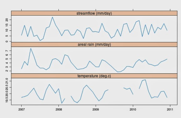
Then ordering your data in monthly basis and plot it.
monthlyPQE <- aggregate(Cikapundung, as.yearmon, mean)
xyplot(monthlyPQE, screens=c("streamflow (mm/day)",
                          "areal rain (mm/day)", "temperature (deg.c)"), xlab=NULL)
Your output should look like this.
You can also check your complete cases and Runoff Ratio (RR)
ok <- complete.cases(Cikapundung[,1:2])
count(ok==T)
sum(Cikapundung$Q[ok])/sum(Cikapundung$P[ok])
The result should be.
     x freq
1 TRUE 1461
and
[1] 0.3672767
Next is calculating the correlation between river discharge (flow) and rainfall with rollccf function and estimating the delay.
r_ccf <- rollccf(Cikapundung)
plot(r_ccf$rolls$"width 365")

# Estimate delay time from rainfall to river
delay <- estimateDelay(Cikapundung)
delay
It should look like this,

and
> delay <- estimateDelay(Cikapundung)
> delay
[1] 2
Now we put in the model spec by defining define data period name ts.cal(calibration period), ts.val, and ts.later as testing period.
ts.cal <- window(Cikapundung,start="2007-01-01",end="2008-12-31")
ts.val <- window(Cikapundung,start="2008-01-01",end="2009-12-31")
ts.later <- window(Cikapundung,start="2009-01-01",end="2010-12-31")
Then defining routing and parameters using:
- ts.cal period
- expuh routing
- cwi (catchment wetness index) as sma (soil moisture accounting)
- tau_s=5-100 (slow flow component),
- tau_q=0-5 (fast flow component),
- v_s=0-1 (fraction volume in slow component)
ckpModel <- hydromad(ts.cal,sma="cwi",routing="expuh",tau_s=c(5,100),tau_q=c(0,5),v_s=c(0,1))
print(ckpModel)
out<-capture.output(print(ckpModel)) # saving result to txt file
cat(out,file="ckpModel1.txt",sep="\n",append=TRUE)
The output should look like this.
Hydromad model with "cwi" SMA and "expuh" routing:
Start = 2007-01-01, End = 2008-12-31

SMA Parameters:
      lower upper
tw        0   100
f         0     8
scale    NA    NA
l         0     0 (==)
p         1     1 (==)
t_ref    20    20 (==)
Routing Parameters:
      lower upper
tau_s     5   100
tau_q     0     5
v_s       0     1
Model calibration using fitByOptim function.
ckpModel <- update(ckpModel, sma="cmd", routing="armax", rfit=list("sriv", order=c(n=2,m=1)))
ckpFit <- fitByOptim(ckpModel, samples=100, method="PORT")
If you get error messages like subset out of bound etc, most likely you have problem with you data (eg: date format etc).
Then we try to simulate other period ts.val and ts.later,
simval <- update(ckpFit, newdata=ts.val)
simlater <- update(ckpFit, newdata=ts.later)
then running verification towhole dataset, excluding calib data.
dataVerif <- Cikapundung # make dataVerif frame from Cotter
dataVerif$Q[time(ts.cal)] <- NA # we verify Q and excluding data90ss
simVerif <- update(ckpFit, newdata=dataVerif) # run dataVerif, save in simVerif
Next we can group all models using runlist function and save it in txt file,
allModels <- runlist(calibration=ckpFit, simval, simlater, simVerif)
summary(allModels) # summary of model performance
print(allModels)
out<-capture.output(print(allModels))
cat(out,file="allModels.txt",sep="\n",append=TRUE)
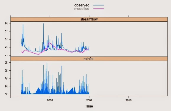
plotting ckpFit with defined period,
xyplot(ckpFit, with.P=TRUE, xlim=as.Date(c("2007-01-01", "2010-12-31")))
It should look like this.

and plotting allModels
xyplot(allModels[2:3], scales = list(y = list(log = TRUE)))
It should look like this.

The allModels summary should look like this.
         rel.bias    r.squared   r.sq.sqrt    r.sq.log
calibration -0.2168151 -0.380018043 -0.60152528 -0.64466581
simval       0.1793397 -0.524916565 -0.68196244 -0.73832646
simlater     0.5275161 -2.195907097 -1.63192686 -1.45632787
simVerif     0.1042556 -0.003519501  0.06358249  0.08402725